CS61a 2023 暑期 学习日记

种种原因,本来说暑假学完 cs61b, 但因为 cs61a 此前没学,于是决定先速通 cs61a
选择的是 fa20, 因为听说这个学期开源的最多

这是个日记贴,按道理来说会每天更新,也是对自己的一个督促

2023-06-25T23:30:00Z2023-06-26T17:00:00Z

先从 Textbook 阅读开始,阅读了 ch1.1, ch1.2, ch1.3, 虽然上个学期自学过 python, 但是大片的英文读的我属实是有点不适应 (感觉语法之类阅读难度都胜于之前读一些文档,, ,).
这样一对比,看完 textbook 再看 videos 就很享受了,20fa 的 John 教授口语十分清晰好听很容易听明白.
然后试了下课程配套的 lab, 很好用孩子很喜欢吃 (bushi

一天下来没写什么东西,倒是十分感叹别人家教学的先进和人性化.

笔记

Expressions

  • Expressions
  • Call Expressions

Name

Name – bind – object

The name of a function is repeated twice, once in the frame and again as part of the function itself. The name appearing in the function is called the intrinsic name. The name in a frame is a bound name.

There is a difference between the two: different names may refer to the same function, but that function itself has only one intrinsic name.

Environment

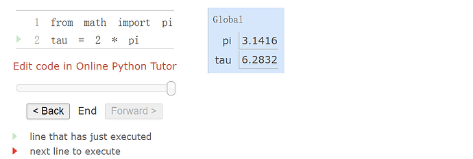
The possibility of binding names to values and later retrieving those values by name means that the interpreter must maintain some sort of memory that keeps track of the names, values, and bindings. This memory is called an environment.

An environment in which an expression is evaluated consists of a sequence of frames.

Each frame contains bindings, each of which associates a name with its corresponding value.

There is a single global frame.

Assignment and import statements add entries to the first frame of the current environment.

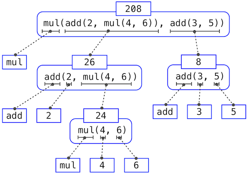
Evaluating Nested Expressions

expression tree:

expression_tree

The Non-Pure Print Function

In addition to returning a value, applying a non-pure function can generate side effects, which make some change to the state of the interpreter or computer. A common side effect is to generate additional output beyond the return value, using the print function.

>>> print(print(1), print(2))
1
2
None None

Calling User-Defined Functions

To evaluate a call expression whose operator names a user-defined function, the Python interpreter follows a computational process. As with any call expression, the interpreter evaluates the operator and operand expressions, and then applies the named function to the resulting arguments.

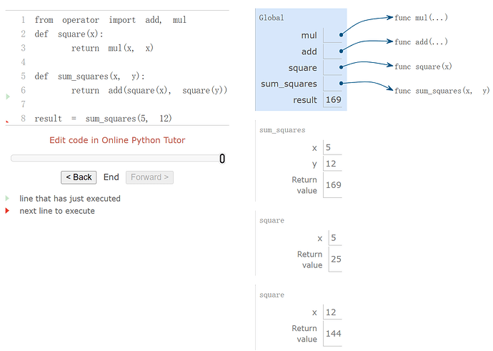
Applying a user-defined function introduces a second local frame, which is only accessible to that function. To apply a user-defined function to some arguments:

  1. Bind the arguments to the names of the function’s formal parameters in a new local frame.
  2. Execute the body of the function in the environment that starts with this frame.

The environment in which the body is evaluated consists of two frames: first the local frame that contains formal parameter bindings, then the global frame that contains everything else. Each instance of a function application has its own independent local frame.

Functions as Abstractions

Aspects of a functional abstraction. To master the use of a functional abstraction, it is often useful to consider its three core attributes. The domain of a function is the set of arguments it can take. The range of a function is the set of values it can return. The intent of a function is the relationship it computes between inputs and output (as well as any side effects it might generate). Understanding functional abstractions via their domain, range, and intent is critical to using them correctly in a complex program.

For example, any square function that we use to implement sum_squares should have these attributes:

  • The domain is any single real number.
  • The range is any non-negative real number.
  • The intent is that the output is the square of the input.

2023-06-27T00:00:00Z2023-06-27T17:00:00Z

今天睡觉睡得很多 (下午从 13:00 睡到 17:00), 有点低效率,只读完了 textbook ch.1.4-ch.1.5, 看完了 lec3 的 videos, 完成了 lab01 和 hw01
照这个速度看速通比较困难,所以明天 (今天早上起来) 开始需要尽可能保持高效才行 :face_exhaling:

笔记

Ch.1.4 Designing Functions

Remember, code is written only once, but often read many times.

Documentation

A function definition will often include documentation describing the function, called a docstring, which must be indented along with the function body. Docstrings are conventionally triple quoted. The first line describes the job of the function in one line. The following lines can describe arguments and clarify the behavior of the function.

Comments in Python can be attached to the end of a line following the # symbol.

Default Argument Values

In Python, we can provide default values for the arguments of a function. When calling that function, arguments with default values are optional. If they are not provided, then the default value is bound to the formal parameter name instead.

As a guideline, most data values used in a function’s body should be expressed as default values to named arguments, so that they are easy to inspect and can be changed by the function caller. Some values that never change, such as the fundamental constant k, can be bound in the function body or in the global frame.

def pressure(v, t, n=6.022e23):
	"""Compute the pressure in pascals of an ideal gas.

    v -- volume of gas, in cubic meters
    t -- absolute temperature in degrees kelvin
    n -- particles of gas (default: one mole)
    """
    k = 1.38e-23  # Boltzmann's constant
    return n * k * t / v
>>> pressure(1, 273.15)
2269.974834
>>> pressure(1, 273.15, 3 * 6.022e23)
6809.924502

Ch.1.5 Control

Statements

At its highest level, the Python interpreter’s job is to execute programs, composed of statements. However, much of the interesting work of computation comes from evaluating expressions. Statements govern the relationship among different expressions in a program and what happens to their results.

Compound Statements

  • A simple statement is a single line that doesn’t end in a colon.
  • A compound statement is so called because it is composed of other statements (simple and compound).

Together, a header and an indented suite of statements is called a clause. A compound statement consists of one or more clauses:

<header>:
    <statement>
    <statement>
    ...
<separating header>:
    <statement>
    <statement>
    ...

We can now know that,

  • Expressions, return statements, and assignment statements are simple statements.
  • A def statement is a compound statement. The suite that follows the def header defines the function body.

We say that the header controls its suite.

Defining Functions II: Local Assignment

The effect of an assignment statement is to bind a name to a value in the first frame of the current environment. As a consequence, assignment statements within a function body cannot affect the global frame.

Conditional Statements

A conditional statement in Python consists of a series of headers and suites: a required if clause, an optional sequence of elif clauses, and finally an optional else clause

There is short-circuiting in Python when executing logical expressions

Functions that perform comparisons and return boolean values typically begin with is, not followed by an underscore (e.g., isfinite, isdigit, isinstance, etc.).

  • not has the highest priority
  • and
  • or has the lowest priority

Iteration

A while clause contains a header expression followed by a suite:

while <expression>:
    <suite>

A while statement that does not terminate is called an infinite loop. Press <Control>-C to force Python to stop looping.

Testing

Assertions

Programmers use assert statements to verify expectations, such as the output of a function being tested. An assert statement has an expression in a boolean context, followed by a quoted line of text (single or double quotes are both fine, but be consistent) that will be displayed if the expression evaluates to a false value.

>>> assert fib(8) == 13, 'The 8th Fibonacci number should be 13'

When the expression being asserted evaluates to a true value, executing an assert statement has no effect. When it is a false value, assert causes an error that halts execution.

A test function for fib should test several arguments, including extreme values of n.

>>> def fib_test():
        assert fib(2) == 1, 'The 2nd Fibonacci number should be 1'
        assert fib(3) == 1, 'The 3rd Fibonacci number should be 1'
        assert fib(50) == 7778742049, 'Error at the 50th Fibonacci number'

When writing Python in files, rather than directly into the interpreter, tests are typically written in the same file or a neighboring file with the suffix _test.py.

Doctests

Python provides a convenient method for placing simple tests directly in the docstring of a function. The first line of a docstring should contain a one-line description of the function, followed by a blank line. A detailed description of arguments and behavior may follow. In addition, the docstring may include a sample interactive session that calls the function:

>>> def sum_naturals(n):
        """Return the sum of the first n natural numbers.

        >>> sum_naturals(10)
        55
        >>> sum_naturals(100)
        5050
        """
        total, k = 0, 1
        while k <= n:
            total, k = total + k, k + 1
        return total

Test all functions:

the interaction can be verified via the doctest module.

>>> from doctest import testmod
>>> testmod()
TestResults(failed=0, attempted=2)

Test one function:

we use a doctest function called run_docstring_examples.

Its first argument is the function to test. The second should always be the result of the expression globals(), a built-in function that returns the global environment. The third argument is True to indicate that we would like “verbose” output: a catalog of all tests run.

>>> from doctest import run_docstring_examples
>>> run_docstring_examples(sum_naturals, globals(), True)
Finding tests in NoName
Trying:
    sum_naturals(10)
Expecting:
    55
ok
Trying:
    sum_naturals(100)
Expecting:
    5050
ok

When writing Python in files, all doctests in a file can be run by starting Python with the doctest command line option:

python3 -m doctest <python_source_file> 
python3 -m doctest -v <python_source_file> 

The key to effective testing is to write (and run) tests immediately after implementing new functions. It is even good practice to write some tests before you implement, in order to have some example inputs and outputs in your mind. A test that applies a single function is called a unit test. Exhaustive unit testing is a hallmark of good program design.

6 Likes

但是我之前除了 The Missing Semester of Your CS Education (mit.edu) 再没接触过别的英文课程,知识方面也是只会做一些题没写过 project. 先从 cs61a 开始一方面满足了我的强迫症 (bushi), 我也想系统的接收知识,一方面可以让我练练英语,一方面可以让我接触一些简单的 project.

还好暑假还长,一个一个来,问题不大!

我可能会学后面自己感兴趣的 ( 上个学期的 c 语言课 我就是在开课后火速跟 mooc 上浙大翁恺老师的课
程序设计入门——C 语言_中国大学 MOOC(慕课) (icourse163.org)
C 语言程序设计进阶_中国大学 MOOC(慕课) (icourse163.org)
学完了课程要求内容,然后继续上浙大的课学数据结构
数据结构_中国大学 MOOC(慕课) (icourse163.org),
期间还学了点 the missing semester 的课

上个学期实践过后感觉这种节奏是我喜欢的 (x

1 Like

我是从 61b 入门的

1 Like

unit test 是好习惯

我才知道这种东西也是会被放到教科书里教给学生的,而且是给刚刚入门计算机的学生们教的。

还有一个有趣的概念叫 Test-Driven Development

在做 cs61a 的 lab01 时,教授提供的 https://inst.eecs.berkeley.edu/~cs61a/fa20/articles/debugging.html 文档就提到了这个:

  • Write some tests before you write code: this is called test-driven development. Writing down how you expect the function to behave first – this can guide you when writing the actual code.
1 Like

2023-06-28T04:00:00Z2023-06-28T17:00:00Z

看了 Debugging | CS 61A Fall 2020 文档 和 噩梦般的 ch.1.6: Higher-Order Functions
看的过程有点痛苦,看到 Newton’s Method 的时候彻底晕了,然后就跳过 Newton’s Method 看完了.
Newton’s Method 到时候看 videos 再说吧
However, 好消息是明天 (今早) 开始可以连续看好多 videos 而不用看书,这是福报啊!!

笔记

Something About The Document: Debugging

Traceback Messages

File "<file name>", line <number>, in <function>

Error Messages

<error type>: <error message>

Debugging Techniques

  • Running doctests

  • Using print statements

    • Long-term debugging

      Sometimes we would like to leave the debugging code if we need to periodically test our file. It can get kind of annoying if every time we run our file, debugging messages pop up. One way to avoid this is to use a global debug variable:

      debug = True
      
      def foo(n):
      i = 0
      while i < n:
          i += func(i)
          if debug:
              print('DEBUG: i is', i)
      
  • Interactive Debugging

    One way a lot of programmers like to investigate their code is by use of an interactive REPL. That is, a terminal where you can directly run functions and inspect their outputs.

    Typically, to accomplish this, you can run

    python -i file.py
    

    and one then has a session of python where all the definitions of file.py have already been executed.

  • Python Tutor Debugging

    Sometimes the best way to understand what is going on with a given piece of python code is to create an environment diagram. While creating an environment diagram by hand can sometimes be tedious, the tool Python Tutor creates environment diagrams automatically.

  • Using assert statements

    For example, if you are writing a function that takes in an integer and doubles it, it might be useful to ensure that your input is in fact an integer. You can then write the following code

    def double(x):
        assert isinstance(x, int), "The input to double(x) must be an integer"
        return 2 * x
    

    Note that we aren’t really debugging the double function here, what we’re doing is ensuring that anyone who calls double is doing so with the right arguments.

    One major benefit of assert statements is that they are more than a debugging tool, you can leave them in code permanantly. A key principle in software development is that it is generally better for code to crash than produce an incorrect result, and having asserts in your code makes it far more likely that your code will crash if it has a bug in it.

Error Types

  • SyntaxError

    This is different from other errors, which are only raised during runtime.

  • IndentationError

  • TypeError

  • NameError

variable not assigned to anything OR it doesn’t exist. This includes function names.

  • IndexError

Lab01 quiz back-up

Q: What is the best way to open an interactive terminal to investigate a failing test for question sum_digits in assignment lab01?
Choose the number of the correct choice:

0) python3 ok -q sum_digits --trace
1) python3 -i lab01.py
2) python3 ok -q sum_digits -i
3) python3 ok -q sum_digits
   ? 2
   -- OK! --

Ch.1.6 Higher-Order Functions

One of the things we should demand from a powerful programming language is the ability to build abstractions by assigning names to common patterns and then to work in terms of the names directly.

Functions that manipulate functions are called higher-order functions.

Functions as Arguments

Using an identity function that returns its argument, we can sum natural numbers using exactly the same summation function.

>>> def summation(n, term):
        total, k = 0, 1
        while k <= n:
            total, k = total + term(k), k + 1
        return total
>>> def identity(x):
        return x
>>> def sum_naturals(n):
        return summation(n, identity)
>>> sum_naturals(10)
55

Functions as General Methods

With higher-order functions, we begin to see a more powerful kind of abstraction: some functions express general methods of computation, independent of the particular functions they call.

When a user-defined function is applied to some arguments, the formal parameters are bound to the values of those arguments (which may be functions) in a new local frame.

Consider the following example, which implements a general method for iterative improvement and uses it to compute the golden ratio. The golden ratio, often called “phi”, is a number near 1.6 that appears frequently in nature, art, and architecture.

An iterative improvement algorithm begins with a guess of a solution to an equation. It repeatedly applies an update function to improve that guess, and applies a close comparison to check whether the current guess is “close enough” to be considered correct.

>>> def improve(update, close, guess=1):
        while not close(guess):
            guess = update(guess)
        return guess

This improve function is a general expression of repetitive refinement. It doesn’t specify what problem is being solved: those details are left to the update and close functions passed in as arguments.

Among the well-known properties of the golden ratio are that it can be computed by repeatedly summing the inverse of any positive number with 1, and that it is one less than its square. We can express these properties as functions to be used with improve.

>>> def golden_update(guess):
        return 1/guess + 1
>>> def square_close_to_successor(guess):
        return approx_eq(guess * guess, guess + 1)

Above, we introduce a call to approx_eq that is meant to return True if its arguments are approximately equal to each other. To implement, approx_eq, we can compare the absolute value of the difference between two numbers to a small tolerance value.

>>> def approx_eq(x, y, tolerance=1e-15):
        return abs(x - y) < tolerance

Calling improve with the arguments golden_update and square_close_to_successor will compute a finite approximation to the golden ratio.

>>> improve(golden_update, square_close_to_successor)
1.6180339887498951

This example illustrates two related big ideas in computer science.

  • First, naming and functions allow us to abstract away a vast amount of complexity. While each function definition has been trivial, the computational process set in motion by our evaluation procedure is quite intricate.
  • Second, it is only by virtue of the fact that we have an extremely general evaluation procedure for the Python language that small components can be composed into complex processes. Understanding the procedure of interpreting programs allows us to validate and inspect the process we have created.

Defining Functions III: Nested Definitions

Let’s consider a new problem: computing the square root of a number. In programming languages, “square root” is often abbreviated as sqrt. Repeated application of the following update converges to the square root of a:

>>> def average(x, y):
        return (x + y)/2
>>> def sqrt_update(x, a):
        return average(x, a/x)

This two-argument update function is incompatible with improve (it takes two arguments, not one), and it provides only a single update, while we really care about taking square roots by repeated updates. The solution to both of these issues is to place function definitions inside the body of other definitions.

>>> def sqrt(a):
        def sqrt_update(x):
            return average(x, a/x)
        def sqrt_close(x):
            return approx_eq(x * x, a)
        return improve(sqrt_update, sqrt_close)

Lexical scope:

Locally defined functions also have access to the name bindings in the scope in which they are defined. In this example, sqrt_update refers to the name a, which is a formal parameter of its enclosing function sqrt. This discipline of sharing names among nested definitions is called lexical scoping. Critically, the inner functions have access to the names in the environment where they are defined (not where they are called).

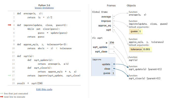
We require two extensions to our environment model to enable lexical scoping.

  1. Each user-defined function has a parent environment: the environment in which it was defined.
  2. When a user-defined function is called, its local frame extends its parent environment.

Previous to sqrt, all functions were defined in the global environment, and so they all had the same parent: the global environment. By contrast, when Python evaluates the first two clauses of sqrt, it create functions that are associated with a local environment.

Only after calling sqrt(a), sqrt_update and sqrt_close will be defined

Function values each have a new annotation that we will include in environment diagrams from now on, a parent. The parent of a function value is the first frame of the environment in which that function was defined. Functions without parent annotations were defined in the global environment. When a user-defined function is called, the frame created has the same parent as that function.

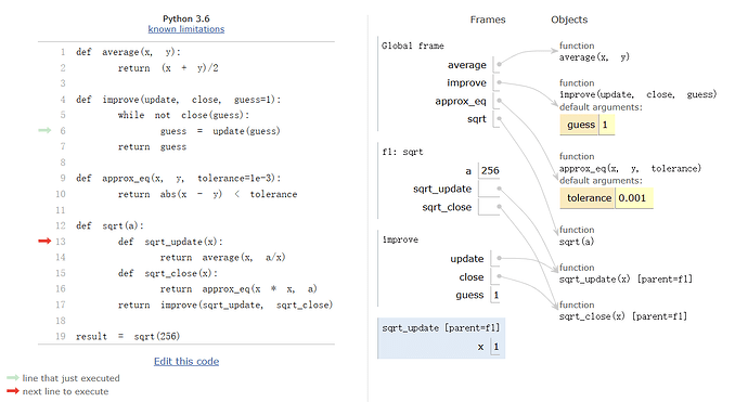
The most critical part of this evaluation procedure is the transfer of the parent for sqrt_updateand sqrt_close to the frame created by calling sqrt_update. This frame is also annotated with [parent=f1].

Extended Environments:

An environment can consist of an arbitrarily long chain of frames, which always concludes with the global frame. Previous to this sqrt example, environments had at most two frames: a local frame and the global frame. By calling functions that were defined within other functions, via nested def statements, we can create longer chains. The environment for this call to sqrt_update consists of three frames: the local sqrt_update frame, the sqrt frame in which sqrt_update was defined (labeled f1), and the global frame.

The return expression in the body of sqrt_update can resolve a value for a by following this chain of frames. Looking up a name finds the first value bound to that name in the current environment. Python checks first in the sqrt_update frame – no a exists. Python checks next in the parent frame, f1, and finds a binding for a to 256.

Hence, we realize two key advantages of lexical scoping in Python.

  • The names of a local function do not interfere with names external to the function in which it is defined, because the local function name will be bound in the current local environment in which it was defined, rather than the global environment.
  • A local function can access the environment of the enclosing function, because the body of the local function is evaluated in an environment that extends the evaluation environment in which it was defined.

The sqrt_update function carries with it some data: the value for a referenced in the environment in which it was defined. Because they “enclose” information in this way, locally defined functions are often called closures.

Functions as Returned Values

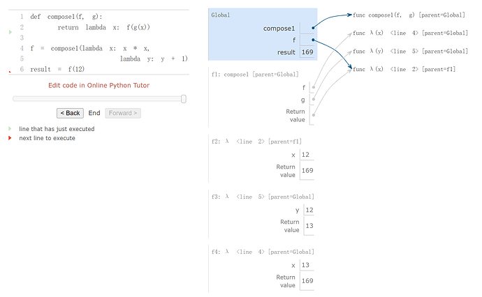
Once many simple functions are defined, function composition is a natural method of combination to include in our programming language. That is, given two functions f(x) and g(x), we might want to define h(x) = f(g(x)). We can define function composition using our existing tools:

>>> def compose1(f, g):
        def h(x):
            return f(g(x))
        return h

The 1 in compose1 is meant to signify that the composed functions all take a single argument. This naming convention is not enforced by the interpreter; the 1 is just part of the function name.

Example: Newton’s Method

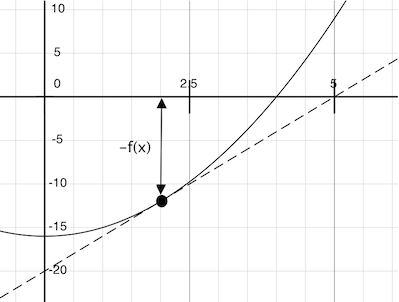
Newton’s method is an iterative improvement algorithm: it improves a guess of the zero for any function that is differentiable, which means that it can be approximated by a straight line at any point. Newton’s method follows these linear approximations to find function zeros.

newton

Imagine a line through the point (x,f(x)) that has the same slope as the curve for function f(x) at that point. Such a line is called the tangent, and its slope is called the derivative of f(x) at x.

Hence, translating x by f(x) divided by the slope will give the argument value at which this tangent line touches 0.

A newton_update expresses the computational process of following this tangent line to 0, for a function f and its derivative df.

后面看课本没看懂了,到时候再看 videos 吧

TODO

Currying

We can use higher-order functions to convert a function that takes multiple arguments into a chain of functions that each take a single argument.More specifically, given a function f(x, y), we can define a function g such that g(x)(y) is equivalent to f(x, y). Here, g is a higher-order function that takes in a single argument x and returns another function that takes in a single argument y. This transformation is called currying.

As an example, we can define a curried version of the pow function:

>>> def curried_pow(x):
        def h(y):
            return pow(x, y)
        return h
>>> curried_pow(2)(3)
8

we manually performed the currying transformation on the pow function to obtain curried_pow. Instead, we can define functions to automate currying, as well as the inverse uncurrying transformation:

>>> def curry2(f):
        """Return a curried version of the given two-argument function."""
        def g(x):
            def h(y):
                return f(x, y)
            return h
        return g
>>> def uncurry2(g):
        """Return a two-argument version of the given curried function."""
        def f(x, y):
            return g(x)(y)
        return f

>>> # can be more concise using lambda expressions introduced later
>>> curry2 = lambda f: (lambda x: (lambda y: f(x, y)))
>>> uncurry2 = lambda f: (lambda x,y: f(x)(y))

>>> pow_curried = curry2(pow)
>>> pow_curried(2)(5)
32
>>> map_to_range(0, 10, pow_curried(2))
1
2
4
8
16
32
64
128
256
512

Lambda Expressions

We can understand the structure of a lambda expression by constructing a corresponding English sentence:

     lambda            x            :          f(g(x))
"A function that    takes x    and returns     f(g(x))"

In general, Python style prefers explicit def statements to lambda expressions, but allows them in cases where a simple function is needed as an argument or return value.

Abstractions and First-Class Functions

The significance of higher-order functions is that they enable us to represent these abstractions explicitly as elements in our programming language, so that they can be handled just like other computational elements.

In general, programming languages impose restrictions on the ways in which computational elements can be manipulated. Elements with the fewest restrictions are said to have first-class status. Some of the “rights and privileges” of first-class elements are:

  1. They may be bound to names.
  2. They may be passed as arguments to functions.
  3. They may be returned as the results of functions.
  4. They may be included in data structures.

Python awards functions full first-class status, and the resulting gain in expressive power is enormous.

这个好有趣,反复观摩感觉好美

square = lambda x: x*x

def search(y):
    """Search x until y(x) is true. x must be a positive int"""
    x = 1
    while True:
        if y(x):
            return x
        x += 1

def inverse(f):
    """return g(y) that g(f(x)) == x
    >>> sqrt = inverse(square)
    >>> sqrt(16)
    4
    """
    return lambda y: search(lambda x: f(x) == y)

函数式编程可用 filter 消除控制流

import itertools

def inverse(f):
    """return g(y) that g(f(x)) == x
    >>> sqrt = inverse(lambda x: x*x)
    >>> sqrt(16)
    4
    """
    return lambda y: next(filter(lambda x: f(x) == y, itertools.count()))
1 Like

每次看到 1000+ days 都难绷
这次是 1024 days
好吉利的数字啊

2023-07-05T13:00:00Z2023-07-06T18:00:00Z

之前几天因为有各种事情摆了什么也没学
然后这近 30 个小时主要就是完成了 project1: hog, 其实就是简单的代码填充,不过还是很有趣的

另外为了解释为什么要学 high order function, 教授还举了不少 function examples
有个比较有趣的是这个生成 .wav 的程序

from wave import open
from struct import Struct
from math import floor

frame_rate = 11025

def encode(x):
    """Encode float x between -1 and 1 as two bytes.
    (See https://docs.python.org/3/library/struct.html)
    """
    i = int(16384 * x)
    return Struct('h').pack(i)

def play(sampler, name='song.wav', seconds=2):
    """Write the output of a sampler function as a wav file.
    (See https://docs.python.org/3/library/wave.html)
    """
    out = open(name, 'wb')
    out.setnchannels(1)
    out.setsampwidth(2)
    out.setframerate(frame_rate)
    t = 0
    while t < seconds * frame_rate:
        sample = sampler(t)
        out.writeframes(encode(sample))
        t = t + 1
    out.close()

def tri(frequency, amplitude=0.3):
    """A continuous triangle wave."""
    period = frame_rate // frequency    # 1 个周期中有 period 个采样点
    def sampler(t):
        saw_wave = t / period - floor(t / period + 0.5)
        tri_wave = 2 * abs(2 * saw_wave) - 1
        return amplitude * tri_wave
    return sampler

c_freq, e_freq, g_freq = 261.63, 329.63, 392.00
c = tri(c_freq)
e = tri(e_freq)
g = tri(g_freq)
low_g = tri(g_freq / 2)

def both(f, g):
    return lambda t: f(t) + g(t)

def note(f, start, end, fade=0.01):
    """Play f for a fixed duration."""
    def sampler(t):
        seconds = t / frame_rate
        if seconds < start:
            return 0
        elif seconds > end:
            return 0
        elif seconds < start + fade:
            return (seconds - start) / fade * f(t)
        elif seconds > end - fade:
            return (end - seconds) / fade * f(t)
        else:
            return f(t)
    return sampler

def mario(c, e, g, low_g):
    z = 0
    song = note(e, z, z + 1/8)
    z += 1/8
    song = both(song, note(e, z, z + 1/8))
    z += 1/4
    song = both(song, note(e, z, z + 1/8))
    z += 1/4
    song = both(song, note(c, z, z + 1/8))
    z += 1/8
    song = both(song, note(e, z, z + 1/8))
    z += 1/4
    song = both(song, note(g, z, z + 1/4))
    z += 1/2
    song = both(song, note(low_g, z, z + 1/4))
    return song

def mario_at(octave):
    c = tri(octave * c_freq)
    e = tri(octave * e_freq)
    g = tri(octave * g_freq)
    low_g = tri(octave * g_freq / 2)
    return mario(c, e, g, low_g)

play(both(mario_at(1), mario_at(1/2)))

^这段可以成功生成马里奥的开场音乐

1 Like

2023-07-07T16:00:00Z2023-07-09T04:00:00Z

讲的是 recursion, 讲的比较基础,书看完视频看完就过了,明天开始军训,希望能继续学.

笔记

Ch.1.7 Recursive Functions

A simple recursive function:

def sum_digits(n):
    """Return the sum of the digits of positive integer n."""
    if n < 10:
        return n
    else:
        all_but_last, last = n // 10, n % 10
    	return sum_digits(all_but_last) + last

The Anatomy of Recursive Functions

Treating a recursive call as a functional abstraction has been called a recursive leap of faith. We define a function in terms of itself, but simply trust that the simpler cases will work correctly when verifying the correctness of the function.

Mutual Recursion

When a recursive procedure is divided among two functions that call each other, the functions are said to be mutually recursive. As an example, consider the following definition of even and odd for non-negative integers:

  • a number is even if it is one more than an odd number
  • a number is odd if it is one more than an even number
  • 0 is even

Using this definition, we can implement mutually recursive functions to determine whether a number is even or odd:

def is_even(n):
    if n == 0:
        return True
    else:
        return is_odd(n-1)
    
def is_odd(n):
    if n == 0:
        return False
    else:
        return is_even(n-1)

Mutually recursive functions can be turned into a single recursive function by breaking the abstraction boundary between the two functions.

def is_even(n):
    if n == 0:
        return True
    else:
        if (n-1) == 0:
            return False
        else:
            return is_even((n-1)-1)

Printing in Recursive Functions

def cascade(n):
    """Print a cascade of prefixes of n.
    >>> cascade(1234)
    1234
    123
    12
    1
    12
    123
    1234
    """
    if n < 10:
        print(n)
    else:
        print(n)
        cascade(n//10)
        print(n)
# this function can be expressed more compactly by observing that 
# print(n) is repeated in both clauses of the conditional statement

def cascade(n):
    print(n)
    if n >= 10:
        cascade(n//10)
        print(n)

Then consider a two-player game in which there are n initial pebbles on a table. The players take turns, removing either one or two pebbles from the table, and the player who removes the final pebble wins. Suppose that Alice and Bob play this game, each using a simple strategy:

  • Alice always removes a single pebble
  • Bob removes two pebbles if an even number of pebbles is on the table, and one otherwise

Given n initial pebbles and Alice starting, who wins the game?

A natural decomposition of this problem is to encapsulate each strategy in its own function. This allows us to modify one strategy without affecting the other, maintaining the abstraction barrier between the two. In order to incorporate the turn-by-turn nature of the game, these two functions call each other at the end of each turn.

def play_alice(n):
    if n == 0:
        print("Bob wins!")
    else:
        play_bob(n-1)
def play_bob(n):
    if n == 0:
        print("Alice wins!")
    elif n % 2 == 0:
        play_alice(n-2)
    else:
        play_alice(n-1)

Tree Recursion

Another common pattern of computation is called tree recursion, in which a function calls itself more than once. As an example, consider computing the sequence of Fibonacci numbers, in which each number is the sum of the preceding two.

def fib(n):
    if n == 1:
        return 0
    if n == 2:
        return 1
    else:
        return fib(n-2) + fib(n-1)

Example: Partitions

The number of partitions of a positive integer n, using parts up to size m, is the number of ways in which n can be expressed as the sum of positive integer parts up to m in increasing order.

The number of ways to partition n using integers up to m equals

  1. the number of ways to partition n-m using integers up to m, and
  2. the number of ways to partition n using integers up to m-1.

To see why this is true, observe that all the ways of partitioning n can be divided into two groups: those that include at least one m and those that do not. Moreover, each partition in the first group is a partition of n-m, followed by m added at the end. In the example above, the first two partitions contain 4, and the rest do not.

Therefore, we can recursively reduce the problem of partitioning n using integers up to m into two simpler problems: (1) partition a smaller number n-m, and (2) partition with smaller components up to m-1.

To complete the implementation, we need to specify the following base cases:

  1. There is one way to partition 0: include no parts.
  2. There are 0 ways to partition a negative n.
  3. There are 0 ways to partition any n greater than 0 using parts of size 0 or less.
def count_partitions(n, m):
    """Count the ways to partition n using parts up to m."""
    if n == 0:
        return 1
    elif n < 0:
        return 0
    elif m == 0:
        return 0
    else:
        return count_partitions(n-m, m) + count_partitions(n, m-1)

We can think of a tree-recursive function as exploring different possibilities. In this case, we explore the possibility that we use a part of size m and the possibility that we do not. The first and second recursive calls correspond to these possibilities.

时隔好久又回来了,说说最近干了什么吧:

7 月 28 日回复:然后军训期间我一直在间隙性玉玉,什么都没干

军训后狠狠现充了几天,然后前几天一直在对着 mdn 学前端,目前学了 guides 里面的 html 和 css, js 只了解了 web 入门 里的那点东西。之后计划和 cs61a 同步推进

然后今天把 cs61a chapter 1 彻底结束了。明天希望可以再干点事情

最近在看教材,记了点笔记,感觉难度一般就没怎么更新 另外最近在看前端三大件 ## Ch.2.1 Introduction

Every value in Python has a class that determines what type of value it is. Values that share a class also share behavior. For example, the integers 1 and 2 are both instances of the int class.

Python includes three native numeric types: integers (int), real numbers (float), and complex numbers (complex).

>>> type(1.5)
<class 'float'>
>>> type(1+1j)
<class 'complex'>

Floats

In particular, int objects represent integers exactly, without any approximation or limits on their size. On the other hand, float objects can represent a wide range of fractional numbers, but not all numbers can be represented exactly, and there are minimum and maximum values. Therefore, float values should be treated as approximations to real values.

>>> 7 / 3 * 3
7.0
>>> 1 / 3 * 7 * 3
6.999999999999999

Ch.2.2 Data Abstraction

The general technique of isolating the parts of a program that deal with how data are represented from the parts that deal with how data are manipulated is a powerful design methodology called data abstraction.

Example: Rational Numbers

A rational number is a ratio of integers, and rational numbers constitute an important sub-class of real numbers. A rational number such as 1/3 or 17/29 is typically written as:

<numerator>/<denominator>

where both the <numerator> and <denominator> are placeholders for integer values.

Actually dividing integers produces a float approximation, losing the exact precision of integers. However, we can create an exact representation for rational numbers by combining together the numerator and denominator.

  • rational(n, d) returns the rational number with numerator n and denominator d.
  • numer(x) returns the numerator of the rational number x.
  • denom(x) returns the denominator of the rational number x.

We are using here a powerful strategy for designing programs: wishful thinking. We haven’t yet said how a rational number is represented, or how the functions numer, denom, and rational should be implemented. Even so, if we did define these three functions, we could then add, multiply, print, and test equality of rational numbers:

>>> def add_rationals(x, y):
        nx, dx = numer(x), denom(x)
        ny, dy = numer(y), denom(y)
        return rational(nx * dy + ny * dx, dx * dy)
>>> def mul_rationals(x, y):
        return rational(numer(x) * numer(y), denom(x) * denom(y))
>>> def print_rational(x):
        print(numer(x), '/', denom(x))
>>> def rationals_are_equal(x, y):
        return numer(x) * denom(y) == numer(y) * denom(x)

Now we have the operations on rational numbers defined in terms of the selector functions numer and denom, and the constructor function rational, but we haven’t yet defined these functions. What we need is some way to glue together a numerator and a denominator into a compound value.

Pairs

Unpack a list into its elements and binds each element to a different name

>>> pair = [10, 20]
>>> x, y = pair
>>> x
10
>>> y
20

Two-element lists are not the only method of representing pairs in Python. Any way of bundling two values together into one can be considered a pair. Lists are a common method to do so.

We can now represent a rational number as a pair of two integers: a numerator and a denominator.

>>> from fractions import gcd
>>> def rational(n, d):
        g = gcd(n, d)
        return (n//g, d//g)
>>> def numer(x):
        return x[0]
>>> def denom(x):
        return x[1]

Together with the arithmetic operations we defined earlier, we can manipulate rational numbers with the functions we have defined.

This improvement was accomplished by changing the constructor without changing any of the functions that implement the actual arithmetic operations.

Abstraction Barriers

An abstraction barrier violation occurs whenever a part of the program that can use a higher level function instead uses a function in a lower level. For example, a function that computes the square of a rational number is best implemented in terms of mul_rational, which does not assume anything about the implementation of a rational number.

>>> def square_rational(x):
        return mul_rational(x, x)

Referring directly to numerators and denominators would violate one abstraction barrier.

>>> def square_rational_violating_once(x):
        return rational(numer(x) * numer(x), denom(x) * denom(x))

Assuming that rationals are represented as two-element lists would violate two abstraction barriers.

>>> def square_rational_violating_twice(x):
        return [x[0] * x[0], x[1] * x[1]]

Abstraction barriers make programs easier to maintain and to modify. The fewer functions that depend on a particular representation, the fewer changes are required when one wants to change that representation. All of these implementations of square_rational have the correct behavior, but only the first is robust to future changes. The square_rational function would not require updating even if we altered the representation of rational numbers. By contrast, square_rational_violating_once would need to be changed whenever the selector or constructor signatures changed, and square_rational_violating_twice would require updating whenever the implementation of rational numbers changed.

The Properties of Data

Abstraction barriers shape the way in which we think about data. A valid representation of a rational number is not restricted to any particular implementation (such as a two-element list); it is a value returned by rational that can be passed to numer, and denom. In addition, the appropriate relationship must hold among the constructor and selectors. That is, if we construct a rational number x from integers n and d, then it should be the case that numer(x)/denom(x) is equal to n/d.

This point of view can be applied broadly, including to the pair values that we used to implement rational numbers. We never actually said much about what a pair was, only that the language supplied the means to create and manipulate lists with two elements. The behavior we require to implement a pair is that it glues two values together. Stated as a behavior condition,

  • If a pair p was constructed from values x and y, then select(p, 0) returns x, and select(p, 1) returns y.

We don’t actually need the list type to create pairs. Instead, we can implement two functions pair and select that fulfill this description just as well as a two-element list.

>>> def pair(x, y):
        """Return a function that represents a pair."""
        def get(index):
            if index == 0:
                return x
            elif index == 1:
                return y
        return get
>>> def select(p, i):
        """Return the element at index i of pair p."""
        return p(i)

With this implementation, we can create and manipulate pairs.

>>> p = pair(20, 14)
>>> select(p, 0)
20
>>> select(p, 1)
14

Ch.2.3 Sequences

Sequences are not instances of a particular built-in type or abstract data representation, but instead a collection of behaviors that are shared among several different types of data.

Lists

>>> digits = [1, 8, 2, 8]
>>> len(digits)
4
>>> digits[3]
8
>>> [2, 7] + digits * 2
[2, 7, 1, 8, 2, 8, 1, 8, 2, 8]
# Any values can be included in a list, including another list.
>>> pairs = [[10, 20], [30, 40]]
>>> pairs[1]
[30, 40]
>>> pairs[1][0]
30

Sequence Iteration

The Python for statement can simplify the while loop which can traversal the whole list by iterating over the element values directly without introducing the name index at all.

>>> def count(s, value):
        """Count the number of occurrences of value in sequence s."""
        total = 0
        for elem in s:
            if elem == value:
                total = total + 1
        return total
>>> count(digits, 8)
2

A for statement consists of a single clause with the form:

for <name> in <expression>:
    <suite>

A for statement is executed by the following procedure:

  1. Evaluate the header <expression>, which must yield an iterable value.
  2. For each element value in that iterable value, in order:
    1. Bind <name> to that value in the current frame.
    2. Execute the <suite>.

This execution procedure refers to iterable values. Lists are a type of sequence, and sequences are iterable values. Their elements are considered in their sequential order. Python includes other iterable types, but we will focus on sequences for now

Sequence unpacking

A common pattern in programs is to have a sequence of elements that are themselves sequences, but all of a fixed length. A for statement may include multiple names in its header to “unpack” each element sequence into its respective elements.

>>> pairs = [[1, 2], [2, 2], [2, 3], [4, 4]]

and wish to find the number of these pairs that have the same first and second element.

>>> same_count = 0

The following for statement with two names in its header will bind each name x and y to the first and second elements in each pair, respectively.

>>> for x, y in pairs:
        if x == y:
            same_count = same_count + 1
>>> same_count
2

Ranges

A range is another built-in type of sequence in Python, which represents a range of integers. Ranges are created with range, which takes two integer arguments: the first number and one beyond the last number in the desired range.

>>> range(1, 10)  # Includes 1, but not 10
range(1, 10)
>>> type(range(1, 10))
<class 'range'>

Calling the list constructor on a range evaluates to a list with the same elements as the range, so that the elements can be easily inspected.

>>> list(range(5, 8))
[5, 6, 7]

If only one argument is given, it is interpreted as one beyond the last value for a range that starts at 0.

>>> list(range(4))
[0, 1, 2, 3]

Ranges commonly appear as the expression in a for header to specify the number of times that the suite should be executed: A common convention is to use a single underscore character for the name in the for header if the name is unused in the suite:

>>> for _ in range(3):
        print('Go Bears!')

Sequence Processing

List Comprehensions

Many sequence processing operations can be expressed by evaluating a fixed expression for each element in a sequence and collecting the resulting values in a result sequence. In Python, a list comprehension is an expression that performs such a computation.

>>> odds = [1, 3, 5, 7, 9]
>>> [x+1 for x in odds]
[2, 4, 6, 8, 10]

Another common sequence processing operation is to select a subset of values that satisfy some condition.

>>> [x for x in odds if 25 % x == 0]
[1, 5]

The general form of a list comprehension is:

[<map expression> for <name> in <sequence expression> if <filter expression>]

Aggregation

A third common pattern in sequence processing is to aggregate all values in a sequence into a single value. The built-in functions sum, min, and max are all examples of aggregation functions.

By combining the patterns of evaluating an expression for each element, selecting a subset of elements, and aggregating elements, we can solve problems using a sequence processing approach.

A perfect number is a positive integer that is equal to the sum of its divisors. The divisors of n are positive integers less than n that divide evenly into n. Listing the divisors of n can be expressed with a list comprehension.

>>> def divisors(n):
     return [1] + [x for x in range(2, n) if n % x == 0]
>>> divisors(4)
[1, 2]
>>> divisors(12)
[1, 2, 3, 4, 6]

Using divisors, we can compute all perfect numbers from 1 to 1000 with another list comprehension. (1 is typically considered to be a perfect number as well, but it does not qualify under our definition of divisors.)

>>> [n for n in range(1, 1000) if sum(divisors(n)) == n]
[6, 28, 496]

Higher-Order Functions

Many forms of aggregation can be expressed as repeatedly applying a two-argument function to the reduced value so far and each element in turn.

>>> def reduce(reduce_fn, s, initial):
        reduced = initial
        for x in s:
            reduced = reduce_fn(reduced, x)
        return reduced

For example, reduce can be used to multiply together all elements of a sequence. Using mul as the reduce_fn and 1 as the initial value, reduce can be used to multiply together a sequence of numbers.

Conventional Names

In Python, the built-in map and filter are generalizations of these functions that do not return lists. These functions are discussed in Chapter 4. The definitions above are equivalent to applying the list constructor to the result of built-in map and filter calls.

>>> apply_to_all = lambda map_fn, s: list(map(map_fn, s))
>>> keep_if = lambda filter_fn, s: list(filter(filter_fn, s))

The reduce function is built into the functools module of the Python standard library. In this version, the initial argument is optional.

>>> from functools import reduce
>>> from operator import mul
>>> def product(s):
        return reduce(mul, s)
>>> product([1, 2, 3, 4, 5])
120

Sequence Abstraction

We have introduced two native data types that satisfy the sequence abstraction: lists and ranges. Both satisfy the conditions with which we began this section: length and element selection. Python includes two more behaviors of sequence types that extend the sequence abstraction.

Membership

Python has two operators in and not in that evaluate to True or False depending on whether an element appears in a sequence

Slicing

A slice of a sequence is any contiguous span of the original sequence, designated by a pair of integers. As with the range constructor, the first integer indicates the starting index of the slice and the second indicates one beyond the ending index.

In Python, sequence slicing is expressed similarly to element selection, using square brackets. A colon separates the starting and ending indices. Any bound that is omitted is assumed to be an extreme value: 0 for the starting index, and the length of the sequence for the ending index.

Strings

The native data type for text in Python is called a string, and corresponds to the constructor str.

  • String literals can express arbitrary text, surrounded by either single or double quotation marks.

    • We have seen strings already in our code, as docstrings, in calls to print, and as error messages in assert statements.
  • Strings satisfy the two basic conditions of a sequence that we introduced at the beginning of this section: they have a length and they support element selection.

  • The elements of a string are themselves strings that have only a single character. A character is any single letter of the alphabet, punctuation mark, or other symbol. Unlike many other programming languages, Python does not have a separate character type; any text is a string, and strings that represent single characters have a length of 1.

  • Like lists, strings can also be combined via addition and multiplication.

Membership

The membership operator in applies to strings, but has an entirely different behavior than when it is applied to sequences. It matches substrings rather than elements.

>>> 'here' in "Where's Waldo?"
True

Multiline Literals

Strings aren’t limited to a single line. Triple quotes delimit string literals that span multiple lines. We have used this triple quoting extensively already for docstrings.

>>> """The Zen of Python
claims, Readability counts.
Read more: import this."""
'The Zen of Python\nclaims, "Readability counts."\nRead more: import this.'

In the printed result above, the \n (pronounced “backslash en”) is a single element that represents a new line. Although it appears as two characters (backslash and “n”), it is considered a single character for the purposes of length and element selection.

String Coercion

A string can be created from any object in Python by calling the str constructor function with an object value as its argument. This feature of strings is useful for constructing descriptive strings from objects of various types.

>>> str(2) + ' is an element of ' + str(digits)
'2 is an element of [1, 8, 2, 8]'

Trees

Our ability to use lists as the elements of other lists provides a new means of combination in our programming language. This ability is called a closure property of a data type. In general, a method for combining data values has a closure property if the result of combination can itself be combined using the same method. Closure is the key to power in any means of combination because it permits us to create hierarchical structures — structures made up of parts, which themselves are made up of parts, and so on.

Nesting lists within lists can introduce complexity. The tree is a fundamental data abstraction that imposes regularity on how hierarchical values are structured and manipulated.

A tree has a root label and a sequence of branches. Each branch of a tree is a tree. A tree with no branches is called a leaf. Any tree contained within a tree is called a sub-tree of that tree (such as a branch of a branch). The root of each sub-tree of a tree is called a node in that tree.

The data abstraction for a tree consists of the constructor tree and the selectors label and branches. We begin with a simplified version.

>>> def tree(root_label, branches=[]):
        for branch in branches:
            assert is_tree(branch), 'branches must be trees'
        return [root_label] + list(branches)
>>> def label(tree):
        return tree[0]
>>> def branches(tree):
        return tree[1:]

A tree is well-formed only if it has a root label and all branches are also trees. The is_tree function is applied in the tree constructor to verify that all branches are well-formed.

>>> def is_tree(tree):
        if type(tree) != list or len(tree) < 1:
            return False
        for branch in branches(tree):
            if not is_tree(branch):
                return False
        return True

The is_leaf function checks whether or not a tree has branches.

>>> def is_leaf(tree):
        return not branches(tree)

Trees can be constructed by nested expressions. The following tree t has root label 3 and two branches.

>>> t = tree(3, [tree(1), tree(2, [tree(1), tree(1)])])
>>> t
[3, [1], [2, [1], [1]]]
>>> label(t)
3
>>> branches(t)
[[1], [2, [1], [1]]]
>>> label(branches(t)[1])
2
>>> is_leaf(t)
False
>>> is_leaf(branches(t)[0])
True

Tree-recursive functions can be used to construct trees. For example, the nth Fibonacci tree has a root label of the nth Fibonacci number and, for n > 1, two branches that are also Fibonacci trees. A Fibonacci tree illustrates the tree-recursive computation of a Fibonacci number.

>>> def fib_tree(n):
        if n == 0 or n == 1:
            return tree(n)
        else:
            left, right = fib_tree(n-2), fib_tree(n-1)
            fib_n = label(left) + label(right)
            return tree(fib_n, [left, right])
>>> fib_tree(5)
[5, [2, [1], [1, [0], [1]]], [3, [1, [0], [1]], [2, [1], [1, [0], [1]]]]]

Tree-recursive functions are also used to process trees. For example, the count_leaves function counts the leaves of a tree.

>>> def count_leaves(tree):
      if is_leaf(tree):
          return 1
      else:
          branch_counts = [count_leaves(b) for b in branches(tree)]
          return sum(branch_counts)
>>> count_leaves(fib_tree(5))
8

Partition trees

Trees can also be used to represent the partitions of an integer. A partition tree for n using parts up to size m is a binary (two branch) tree that represents the choices taken during computation. In a non-leaf partition tree:

  • the left (index 0) branch contains all ways of partitioning n using at least one m,
  • the right (index 1) branch contains partitions using parts up to m-1, and
  • the root label is m.

The labels at the leaves of a partition tree express whether the path from the root of the tree to the leaf represents a successful partition of n.

>>> def partition_tree(n, m):
        """Return a partition tree of n using parts of up to m."""
        if n == 0:
            return tree(True)
        elif n < 0 or m == 0:
            return tree(False)
        else:
            left = partition_tree(n-m, m)
            right = partition_tree(n, m-1)
            return tree(m, [left, right])
>>> partition_tree(2, 2)
[2, [True], [1, [1, [True], [False]], [False]]]

Printing the partitions from a partition tree is another tree-recursive process that traverses the tree, constructing each partition as a list. Whenever a True leaf is reached, the partition is printed.

>>> def print_parts(tree, partition=[]):
        if is_leaf(tree):
            if label(tree):
                print(' + '.join(partition))
        else:
            left, right = branches(tree)
            m = str(label(tree))
            print_parts(left, partition + [m])
            print_parts(right, partition)
>>> print_parts(partition_tree(6, 4))
4 + 2
4 + 1 + 1
3 + 3
3 + 2 + 1
3 + 1 + 1 + 1
2 + 2 + 2
2 + 2 + 1 + 1
2 + 1 + 1 + 1 + 1
1 + 1 + 1 + 1 + 1 + 1

Slicing can be used on the branches of a tree as well. For example, we may want to place a restriction on the number of branches in a tree. A binary tree is either a leaf or a sequence of at most two binary trees. A common tree transformation called binarization computes a binary tree from an original tree by grouping together adjacent branches.

>>> def right_binarize(tree):
        """Construct a right-branching binary tree."""
        if is_leaf(tree):
            return tree
        if len(tree) > 2:
            tree = [tree[0], tree[1:]]
        return [right_binarize(b) for b in tree]
>>> right_binarize([1, 2, 3, 4, 5, 6, 7])
[1, [2, [3, [4, [5, [6, 7]]]]]]

Linked Lists

So far, we have used only native types to represent sequences. However, we can also develop sequence representations that are not built into Python. A common representation of a sequence constructed from nested pairs is called a linked list. The environment diagram below illustrates the linked list representation of a four-element sequence containing 1, 2, 3, and 4.

A linked list is a pair containing the first element of the sequence (in this case 1) and the rest of the sequence (in this case a representation of 2, 3, 4). The second element is also a linked list. The rest of the inner-most linked list containing only 4 is 'empty', a value that represents an empty linked list.

Linked lists have recursive structure: the rest of a linked list is a linked list or 'empty'. We can define an abstract data representation to validate, construct, and select the components of linked lists.

>>> empty = 'empty'
>>> def is_link(s):
        """s is a linked list if it is empty or a (first, rest) pair."""
        return s == empty or (len(s) == 2 and is_link(s[1]))
>>> def link(first, rest):
        """Construct a linked list from its first element and the rest."""
        assert is_link(rest), "rest must be a linked list."
        return [first, rest]
>>> def first(s):
        """Return the first element of a linked list s."""
        assert is_link(s), "first only applies to linked lists."
        assert s != empty, "empty linked list has no first element."
        return s[0]
>>> def rest(s):
        """Return the rest of the elements of a linked list s."""
        assert is_link(s), "rest only applies to linked lists."
        assert s != empty, "empty linked list has no rest."
        return s[1]

Above, link is a constructor and first and rest are selectors for an abstract data representation of linked lists. The behavior condition for a linked list is that, like a pair, its constructor and selectors are inverse functions.

We can use the constructor and selectors to manipulate linked lists.

>>> four = link(1, link(2, link(3, link(4, empty))))
>>> first(four)
1
>>> rest(four)
[2, [3, [4, 'empty']]]

The linked list can store a sequence of values in order, but we have not yet shown that it satisfies the sequence abstraction. Using the abstract data representation we have defined, we can implement the two behaviors that characterize a sequence: length and element selection.

>>> def len_link(s):
        """Return the length of linked list s."""
        length = 0
        while s != empty:
            s, length = rest(s), length + 1
        return length
>>> def getitem_link(s, i):
        """Return the element at index i of linked list s."""
        while i > 0:
            s, i = rest(s), i - 1
        return first(s)
>>> len_link(four)
4
>>> getitem_link(four, 1)
2

Recursive manipulation. Both len_link and getitem_link are iterative. They peel away each layer of nested pair until the end of the list (in len_link) or the desired element (in getitem_link) is reached. We can also implement length and element selection using recursion.

>>> def len_link_recursive(s):
        """Return the length of a linked list s."""
        if s == empty:
            return 0
        return 1 + len_link_recursive(rest(s))
>>> def getitem_link_recursive(s, i):
        """Return the element at index i of linked list s."""
        if i == 0:
            return first(s)
        return getitem_link_recursive(rest(s), i - 1)

Recursion is also useful for transforming and combining linked lists.

>>> def extend_link(s, t):
        """Return a list with the elements of s followed by those of t."""
        assert is_link(s) and is_link(t)
        if s == empty:
            return t
        else:
            return link(first(s), extend_link(rest(s), t))
>>> extend_link(four, four)
[1, [2, [3, [4, [1, [2, [3, [4, 'empty']]]]]]]]
>>> def apply_to_all_link(f, s):
        """Apply f to each element of s."""
        assert is_link(s)
        if s == empty:
            return s
        else:
            return link(f(first(s)), apply_to_all_link(f, rest(s)))
>>> apply_to_all_link(lambda x: x*x, four)
[1, [4, [9, [16, 'empty']]]]
>>> def keep_if_link(f, s):
        """Return a list with elements of s for which f(e) is true."""
        assert is_link(s)
        if s == empty:
            return s
        else:
            kept = keep_if_link(f, rest(s))
            if f(first(s)):
                return link(first(s), kept)
            else:
                return kept
>>> keep_if_link(lambda x: x%2 == 0, four)
[2, [4, 'empty']]
>>> def join_link(s, separator):
        """Return a string of all elements in s separated by separator."""
        if s == empty:
            return ""
        elif rest(s) == empty:
            return str(first(s))
        else:
            return str(first(s)) + separator + join_link(rest(s), separator)
>>> join_link(four, ", ")
'1, 2, 3, 4'
想问一下课程录像怎么看啊,我点进去就要伯克利的账号 :thinking:

Google 一下,有 Youtube Channel 滴:

我看的是 20fall, 这个学期大部分资源都开源了,videos 也可以随便看

最近:
第二章过了一半,做完了第二个 project